Methane transport from the North Sea; comparing gas budgets between top-down and bottom-up approaches
Methane is a potent green house gas and increasing globally in the atmosphere. In the North Sea region methane is being released from natural sources like seeps which are fueled from shallow biogenic gas pockets or deep thermogenic gas reservoirs (Schneider v. Deimling et al., 2011; Mau et al., 2015; Römer et al., 2017), shallow water and intertidal anoxic sediment which temporarily get in direct contact with the atmosphere (Wadden Sea; Grunwald et al., 2009), river runoff from e.g. the Elbe river (Matoušů et al., 2019), but also from about 13,000 abandoned wells (Rehder et al., 1998; Vielstädte et al., 2017).
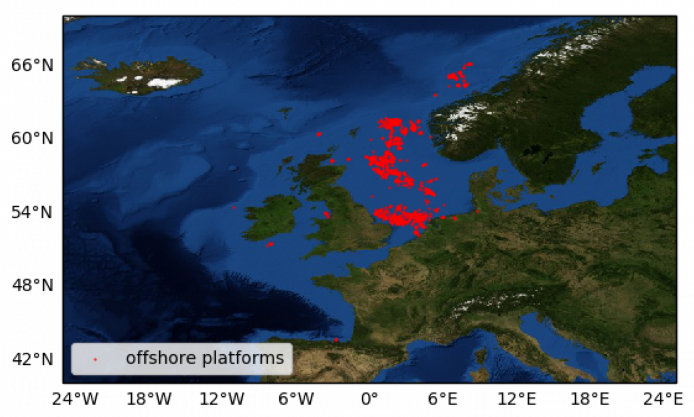
The North Sea is thus a representation of complex and various sources and sinks with internal (supply of gas through faults, biogenic methane generation in sediments) and external (tidal pumping, storm activities, river runoff) forcing. We choose the Methane in the North Sea Region as Show Case as it is a good example for 1) a typical comparison of bottom-up and top-down flux estimates, 2) it demands the compilation of data from various sources, 3) it involves the extrapolation and prediction of data in space and time, 4) and evaluated model/field data and their fit through visual and analytical data exploration. All these are typical generic tasks of data driven science in the marine and atmosphere Earth Sciences which we couple in this Show Case. Following the philosophy of Digital Earth of ‘thinking in workflows’ we divided the overall Show Case in a number of work flows, starting with the compilation of data from various sources (1), perform re-gridding tasks to make spatial data existing as grids comparable in space (2), extrapolate marine free gas release (bubbles) and the related methane flux from abandoned wells into the atmosphere (3), detect patterns in atmospheric data from EDGAR allowing for a better spatial and temporal extrapolation (4), predict the bottom-up methane flux from the North Sea into the atmosphere considering yearly oceanographic and weather variations (5), apply machine learning techniques to predict top-down atmospheric methane concentrations (6), test and use 4D visualization capabilities of the Digital-Earth Viewer (7) to explore data sets (8) and animate currents, fluxes, and comparisons interactively and finally transfer all this into new scientific and technological knowledge. Involved in this Show Case were partners from AWI, GEOMAR, HZG and KIT.
The figure below illustrates the 9 different workflows of the Methane in the North Sea Region Show Case. Click on the different workflows (1 to 9), data inputs (light blue) or approaches and methods (green) to see additional explanations.
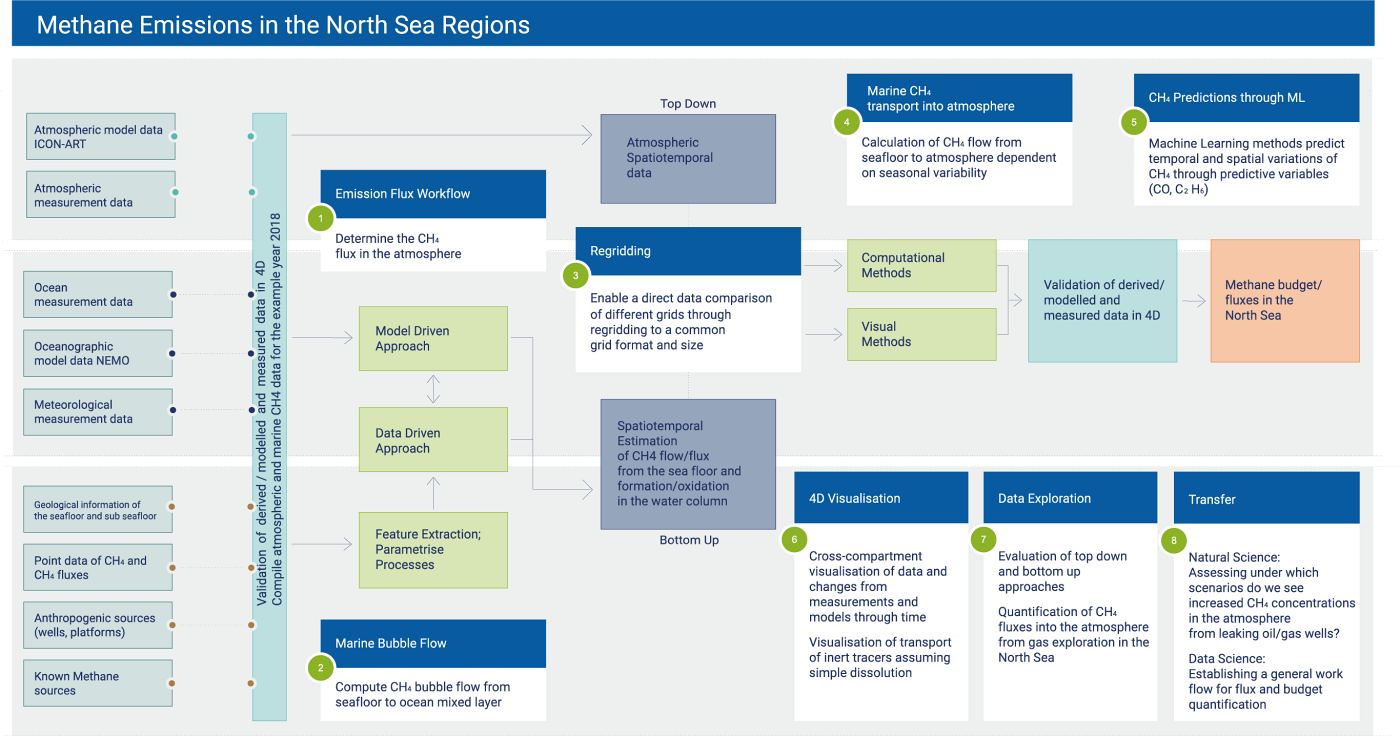
1) Emission Flux Workflow
In this workflow the global model ICON-ART (ICOsahedral Nonhydrostatic model - Aerosols and Reactive Trace gases) is used. ART is an online-coupled model extension for ICON that includes chemical gases and aerosols. Emission data from well established inventories like EDGAR and point information of the OSPAR commission are used as input for the model to simulate the global distribution of trace gases and detect local hotspots. After applying mathematical methods like the Pattern Algorithm on the model data we are going one step further and try to answer the question if emission fluxes can be determined from satellite measurements.
Sentinel 5P
The Copernicus Sentinel-5P (S5P) mission is a collaboration between European Space Agency (ESA) and the Netherlands Space Office (NSO) with the goal to replace current atmospheric monitoring instruments like SCIAMACHY and the Envisat satellite as both come to the end of their lifetimes. The S5P satellite was launched on October 13, 2017 (09:27 GMT) and has an altitude of 824 km with an orbit time of 101 minutes and a repeat cycle of 17 days or 227 orbits. This air quality and atmospheric chemistry monitoring mission aims to track changes in the composition of our earths atmosphere. Sentinel-5P carries the tropospheric measurement instrument TROPOMI, an advanced multispectral imaging spectrometer that scans trace gases like carbon monoxide, formaldehyde, methane, nitrogen dioxide, ozone and aerosols in the atmosphere with a swath width of 2600 km and delivers much information and data on these substances that affect our climate and the air quality.
Find more information and data access here: https://sentinel.esa.int/web/sentinel/missions/sentinel-5p
Reference:
- H. J. Kramer. Copernicus: Sentinel-5p (precursor - atmospheric monitoring mission). https://directory.eoportal.org/web/eoportal/satellite-missions/c-missions/copernicussentinel-5p, Accessed: 2020-07-07, 2020.
OSPAR
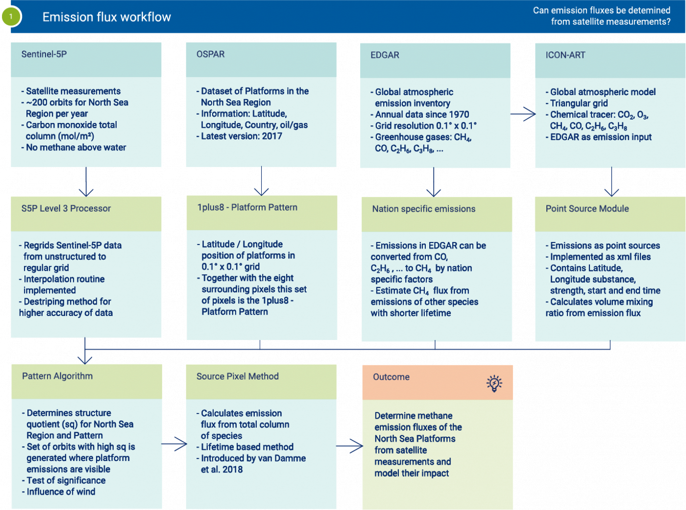
The OSPAR commission has the goal to protect and conserve the North-East Atlantic ocean - in particular the North Sea - and its resources. Starting in 1972 OSPAR monitors the developement of offshore installations and publishes datasets containing the name, ID number, location, operator, water depth, production start, current status, category and function of the platforms. The latest version was published in 2017. The countries with oil and gas industry offshore installations are: Denmark, Germany, Ireland, the Netherlands, Norway, Spain and the United Kingdom. The Figure shows a map of Europe with OSPAR offshore platforms displayed on it.
Find data access here: https://odims.ospar.org/
Reference:
- OSPAR. Offshore Installations. https://www.ospar.org/work-areas/oic/installations, Accessed: 2020-07-07, 2020.
- NASA Visible Earth. https://visibleearth.nasa.gov/collection/1484/blue-marble, Accessed: 2020-07-07, 2020.
Weather Data
The ERA5 dataset is a global weather dataset provided by the European Centre for Medium-Range Weather Forecasts (ECMWF). It covers the atmosphere in 137 levels from the surface level to 80km high. The dataset covers the entire globe using a 30km grid. For our analysis we focus on the year 2018, but data is available since 1979 (1950 in a future release) to near real time. The original dataset provides hourly data, but we use daily aggregated data.
Reference:
- Copernicus Climate Change Service (C3S) (2017): ERA5: Fifth generation of ECMWF atmospheric reanalyses of the global climate . Copernicus Climate Change Service Climate Data Store (CDS). https://cds.climate.copernicus.eu/cdsapp#!/home
EDGAR
The Emission Database for Global Atmospheric Research (EDGAR) is an inventory from the EC-JRC and Netherland’s Environmental Assessment Agency
(Saunois et al., 2016). The EDGARv4.3.2 inventory used as emission input for the simulations in this work covers sector- and country-specific time series of 1970-2012 with monthly resolution and a global spatial resolution of 0.1° x 0.1° providing CH4, CO2, CO, SO2, NOx, C2H6, C3H8 and many other species. The basis for inventories like EDGAR are data from national emission inventory reports that are distributed in space and time via proxy datasets. The latter are based on national spatial data containing information about population density, the road network, waterways, aviation and shipping trajectories. A global 0.1° x 0.1° grid is used on which the emissions are assigned to, either emitted from a single point source (e.g. oil or gas platforms), distributed over a line source (e.g. shiptracks) or over an areal source (e.g. agricultural fields) always depending on the source sectors and subsectors. For this work point sources are from a high importance. These zero-dimensional sources are allocated to a single grid cell of the 0.1° x 0.1° grid with the average of all points that fall into the same cell.
Find more information here: https://edgar.jrc.ec.europa.eu/
Reference:
- G. Janssens-Maenhout, M. Crippa, D. Guizzardi, M. Muntean, E. Schaaf, F. Dentener, P. Bergamaschi, V. Pagliari, J. G. J. Olivier, J. A. H. W. Peters, J. A. Van Aardenne, S. Monni, U. Doering and A. M. R. Petrescu. Edgar v4.3.2 global atlas of the three major greenhouse gas emissions for the period 1970–2012. Earth System Science Data Discussions, 2017:1–55, 2017. doi: 10.5194/essd-2017-79, 2017.
- G. Janssens-Maenhout, V. Pagliari, D. Guizzardi, and M. Muntean. Global emission inventories in the Emission Database for Global Atmospheric Research (EDGAR) Manual (I) Gridding: EDGAR emissions distribution on global gridmaps. European Commission - Joint Research Centre - Institute for Environment and Sustainability, 2012.
ICON-ART
The global model ICON (ICOsahedral Nonhydrostatic model) is a joint development of German Weather Service (DWD) and Max Planck Institute for Meteorology (MPI-M). Due to its dynamical core which is based on the nonhydrostatic formulation of the vertical momentum equation simulations with a high horizontal resolution up to grid spacings of a few hundreds of meters are possible. ART (Aerosols and Reactive Trace Gases) is an online-coupled model extension for ICON that includes chemical gases and aerosols. One aim of the model is the simulation of interactions between the trace substances and the state of the atmosphere by coupling the spatiotemporal evolution of tracers with atmospheric processes.
Find more information here: https://www.dwd.de/DE/forschung/wettervorhersage/nummodellierung/01numvorhersagemodelle/iconbeschreibung.html?nn=19880 https://www.imk-tro.kit.edu/5925.php
Reference:
- Schröter, J., Rieger, D., Stassen, C., Vogel, H., Weimer, M., Werchner, S., Förstner, J., Prill, F., Reinert, D., Zängl, G., Giorgetta, M., Ruhnke, R., Vogel, B., and Braesicke, P.: ICON-ART 2.1: a flexible tracer framework and its application for composition studies in numerical weather forecasting and climate simulations, Geosci. Model Dev., 11, 4043-4068, https://doi.org/10.5194/gmd-11-4043-2018, 2018.
S5P Level 3 Processor
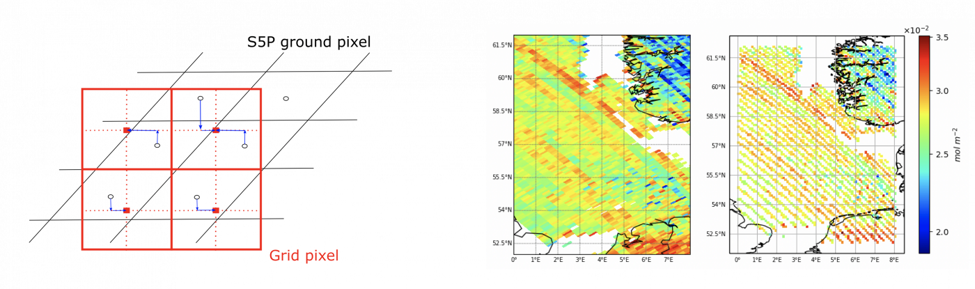
The Sentinel-5P Level-3 processor is a program written in python that processes a unstructured Level-2 product of the TROPOMI spectrometer to regular grid (Level-3 data) and interpolates it as shown in the left Figure. The unstructured parallelograms are displayed in black with their centers as circles. The red squares represent the new structured latitude/longitude grid. Each center of the unstructured parallelograms of the Level-2 data is allocated to exactly one of the Level-3 structured grid centers by first finding the next latitude and then the next longitude that intersects with a new grid center (blue arrows). The right Figure shows that the Sentinel-5P Level-3 processor is mapping the Level-2 data of the TROPOMI instrument in an appropriate way.
Reference:
- European Space Agency. Sentinel-5p. https://sentinel.esa.int/web/sentinel/missions/sentinel-5p, Accessed: 2020-07-07, 2020.
1plus8 - Platform Pattern
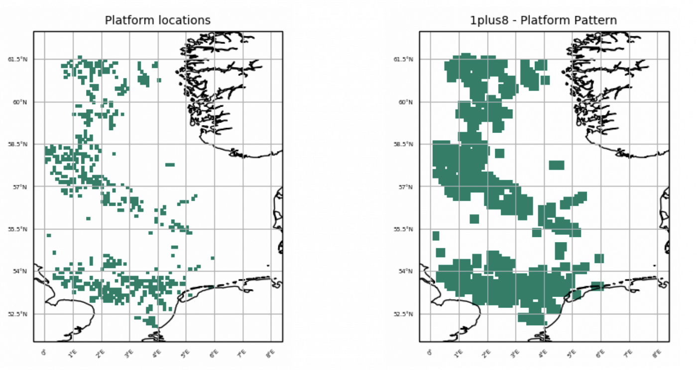
The Latitude / Longitude information of the offshore platforms in the OSPAR dataset are brought to 0.1° x 0.1° grid as displayed in the left Figure. These are the locations where we are about to detect emission fluxes but with respect to transport and other uncertainties we need a larger area around the platforms. Adding the eight surrounding pixels to the platform locations we get the 1plus8 – Platform Pattern as displayed in the right Figure. This is the pattern we are using for the Pattern Algorithm.
Find data access here: https://odims.ospar.org/
Reference:
- OSPAR. Offshore Installations. https://www.ospar.org/work-areas/oic/installations, Accessed: 2020-07-07, 2020.
Point Source Module
The Point Source Module of ART takes given emission fluxes as point sources of substances and adds them to new or existing tracers. Information like Latitude, Longitude, substance, source strength, start and end time are contained in xml files. With the Point Source Module of ART the sensitivity of tracers as well as the temporal and spatial accuracy of emission fluxes are improved.
Reference:
- F. Prill, D. Reiner, D. Rieger, G. Zängl, J. Schröter, J. Förstner, S. Werchner, M. Weimer, R. Ruhnke, and B. Vogel. ICON Model Tutorial. Working with the ICON Model, Practical Exercises for NWP Mode and ICON-ART. Deutscher Wetterdienst, Karlsruhe Institute of Technology, Max-Planck-Institut für Meteorologie, 2019.
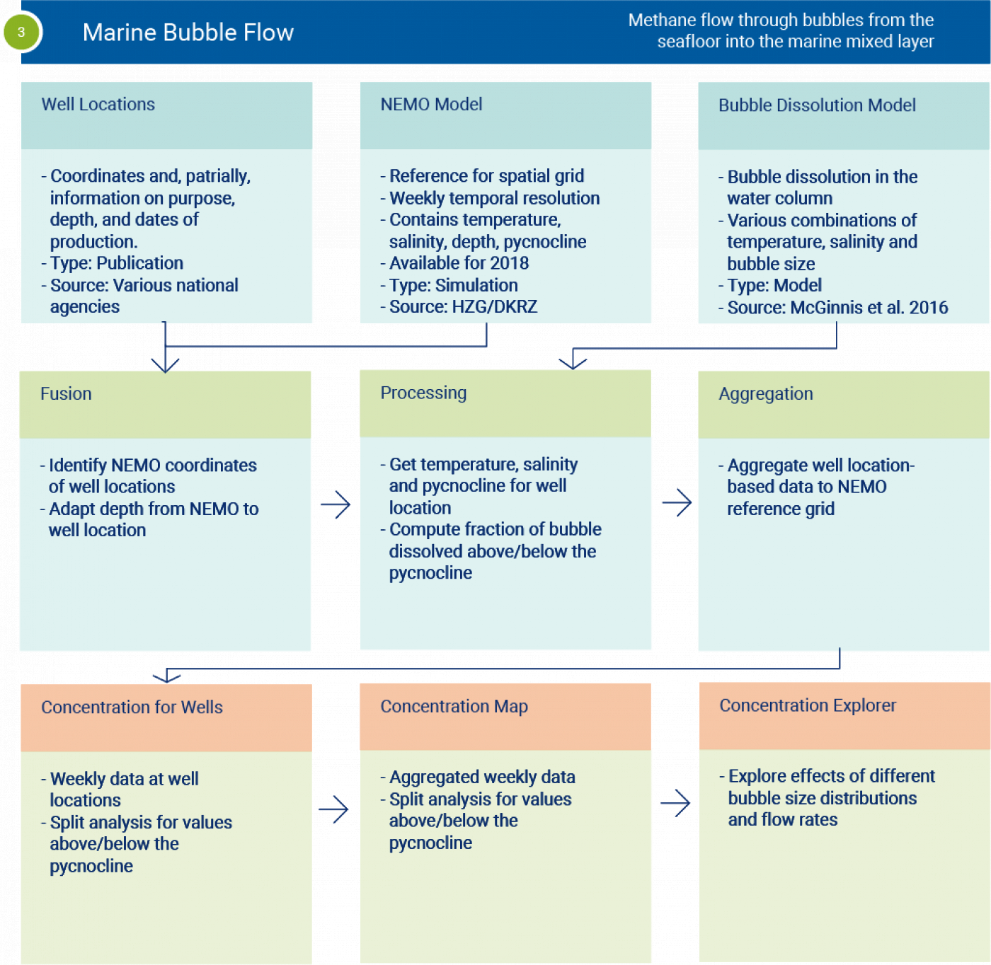
2) Marine Bubble flows
One of the overarching scientific questions is to what extend gas bubble release from the seafloor and specifically from abandoned wells in the North Sea have an impact on atmospheric methane concentrations and how does this change through the seasons. For this evaluation well locations, the change of environmental parameters through a year as well as a bubble dissolution model are needed. Assumptions must be made on e.g. the bubble size distribution (as this determines the rising height and thus transport of methane in the water column) and the absolute amount of gas being released from each well.
Merging the different data sets allows to specify the amount of gas dissolved below the pycnocline and the remaining amount of gas being transported above this atmospheric mixing barrier. The compiled data set allows to interactively manipulate bubble sizes and flow rate at the about 13,000 well locations to see the impact and location of increased gas release towards the atmosphere.
Bubble Dissolution
Methane bubbles, once released from the seafloor, dissolve into the undersaturated water but at the same time strip gases from the water column into the bubble. This means, that the gas composition of the bubbles is changing while the bubble rises (e.g. McGinnis et al., 2006).
Depending on temperature, pressure and salinity gas exchange and equilibrium concentrations change. Knowing the environmental conditions, the initial bubble size and release depth allows to model gas dissolution and the transport of CH4 above the pycnocline where we anticipate full equilibration with the atmosphere - all excess methane from the seafloor that is transported as free gas above the pycnocline will be released into the atmosphere.
We used the GUI-based SingleBubble dissolution software (Greinert & McGinnis, 2009) to calculate bubble dissolution rates for bubbles between 4mm to 12mm diameter, 10m to 220m release depth, salinitiy between 10psu and 36psu and temperature from 2° to 30°C.
Reference:
- Greinert, J. and McGinnis, D.F. (2009): Single Bubble Dissolution Model - The Graphical User Interface SiBu-GUI. Environmental Modelling and Software, 24, 1012-1013, doi:10.1016/j.envsoft.2008.12.011
- McGinnis, D.F., Greinert, J., Artemov, Y., Beaubien, S.E., and Wüest, A. (2006): The fate of rising methane bubbles in stratified waters: What fraction reaches the atmosphere? Journal of Geophysical Research, 111, C09007, doi:10.1029/2005JC003183.

Well Locations
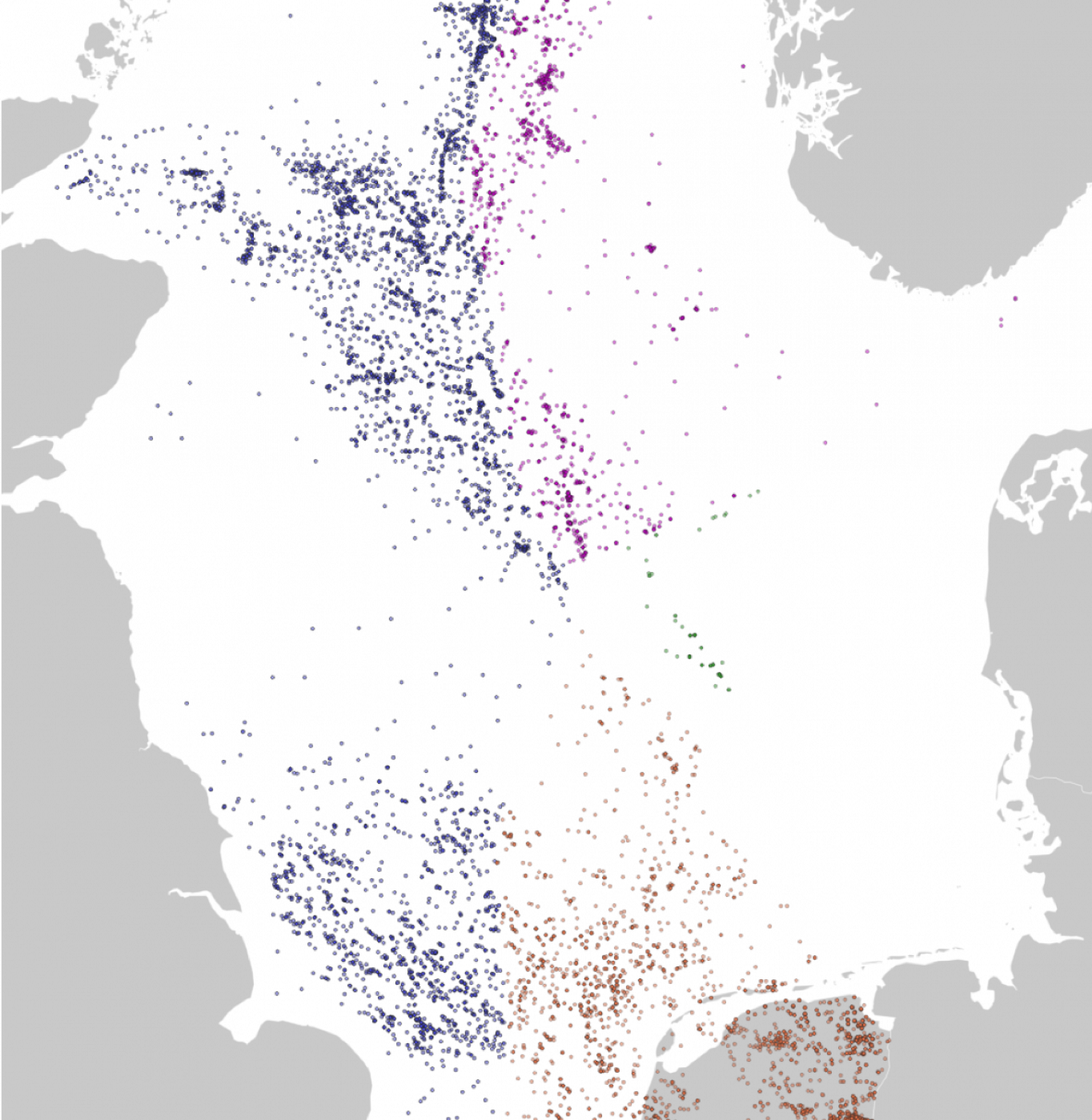
We created a dataset of well locations in the North Sea. The sources of the datasets are the national institutions involved in the regulation of the oil and gas sector in Denmark, the Netherlands, the United Kingdom and Norway. Depending on the source of data, there is information on the depth of the well, the purpose (e.g. exploration for oil or gas, production, …), whether it is active or not, when it was drilled and shut down. Overall there are 22268 wells in our dataset. On the image on the right you can see the individual wells (purple for Norway, blue for the UK, orange for the Netherlands, and green for Denmark).
Reference:
- Danish Energy Agency (https://ens.dk/en/our-responsibilities/oil-gas/about-oil-and-gas)
- NLOG from the Geological Survey of the Netherlands (https://nlog.nl/en/data)
- Oil and Gas Authority UK (https://www.ogauthority.co.uk/data-centre/data-downloads-and-publications/well-data/)
- Norwegian Petroleum Directorate (https://www.npd.no/en/facts/wells/)
NEMO Model
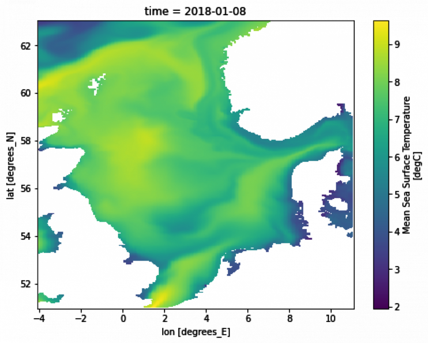
For the properties of the ocean we rely on data from the NEMO model provided by the HZG. Our dataset is a condensed version of the original dataset with adaptions for our use case. The dataset has weekly time steps for our focus year 2018. It covers the North Sea at the original grid cell size. We focus on three depth levels: The surface, the water column above the pycnocline and the water column below the pycnocline. For these levels, the following parameters are provided:
- Temperature
- Salinity
- Zonal current
- Meridional current
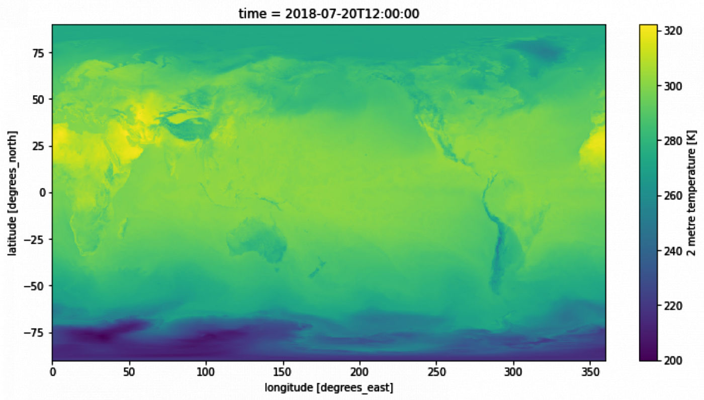
In addition to that, the dataset include the water depth. On the right-hand side you can see a plot of the sea surface temperature for the first week of the year.
Fusion
The first step to create an aggregated map of the methane flow from the ocean floor at well locations is to combined the data on well locations with the data from the NEMO model. Our intention is to create weekly flow rates from the ocean floor to the water column (and the atmosphere; c.f. Processing). To compute the flow rates we need information on the properties of the water column and the water depth at the well locations. The depth is not available for all well location. We therefore use the depth from the NEMO model as a backup solution. Additionally we use the salinity, the temperature and the depth of the pycnocline on a weekly basis from the NEMO model.
These values are collected for all well locations based on the coordinates of the wells. The combined dataset also contains the grid index of the NEMO model for the well locations, because the individual wells will be aggregated to create a map based on the NEMO grid (we use this grid as the reference grid for our workflow).
Processing
We use the bubble dissolution model to calculate the methane flow rates. The model uses the depth at which the bubbles are released together with the properties of the water (salinity and temperature) to calculate dissolution rates for each bubble. The dissolution rates depend on the size of the individual bubbles. We therefore consider multiple bubble sizes:
- 4mm
- 6mm
- 8mm
- 10mm
- 12mm
For each bubble size and each week of the year (the parameters of the water column change, therefore the dissolution rates change as well) we calculate reference values for a flow of one liter per hour. These values for the methane flow to the water column are the aggregate to give values for the flow to water above and below the pycnocline. Because we treat methane above the as going directly to the atmosphere, bubbles reaching the surface are included in the value for the flow to above the pycnocline.
Aggregation
The values calculated so far are for the individual well locations. As the last step, these values need to be aggregated to create a complete map. This map is based on the reference grid from the NEMO model. For each cell with well locations in it, the flow to the water column below and above the pycnocline is calculated. This is done on a weekly basis and for each bubble size independently creating a five-dimensional dataset. Alongside the flow values, information on the well is stored to allow for a future expansion of the „Concentration Explorer“.
A central idea of the aggregation is the preparation of the data in a way that allows testing different bubble size distributions and flow rates (at the well level). This is the core functionality of the „Concentration Explorer“.
Concentration Explorer
The „Concentration Explorer“ is the centerpiece of this workflow. The idea is to allow the user to investigate the influence of different flow rates and bubble size distributions by visualizing the „Flow Map“.
The „Flow Map“ consists of the aggregated well data to the reference grid from the NEMO model. It has two layers for values above and below the pycnocline and holds weekly data for all weeks of 2018. The flow rate can be specified by the user, while the flow can be further configured using a bubble size distribution for which the user has the choice between bubbles sizes 4mm, 6mm, 8mm, 10mm, and 12mm. A time slider can be used to scroll through the weeks of the year.
For the implementation we rely on the „Digital Earth Framework“ which allows us to create a browser-based application.
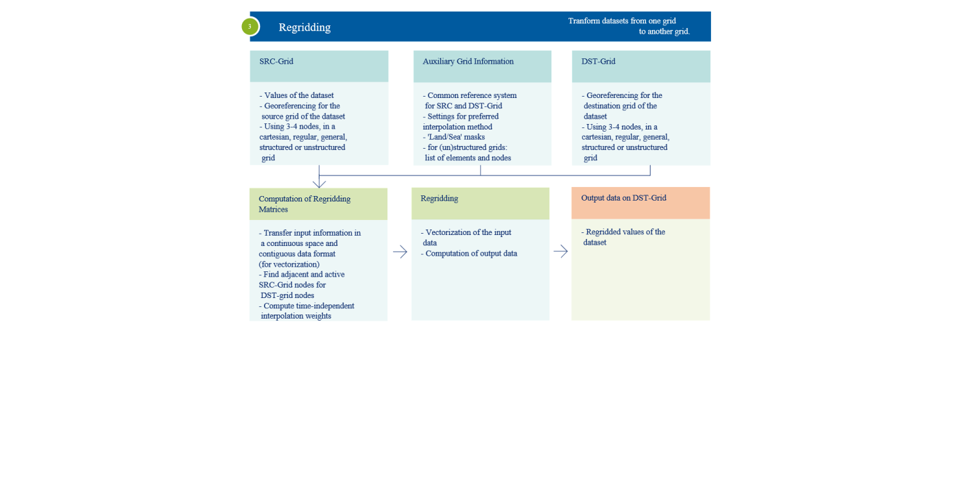
3) Reggriding
Numerical models provide their simulation results on grids, where the values of the dataset are assigned to a finite list of georeferenced positions (nodes). In practice, the values within the space shaped by an adjacent group of nodes (element) are not defined by the gridded results. In order to compare datasets with differing grids, the values within an element can be calculated by functions of the adjacent nodes’ values. The ‘Reggriding’ toolbox provides simple ‚Nearest Neighbor’, bilinear, barocentric and area-weighted conservative regridding for elements consisting of 3-4 nodes with an automatically adapted treatment of masked or missing values. In comparison to other interpolation software packages this are few options, but make it a dependable tool for inexperienced users. Furthermore, the specific programming of the ‘Reggriding’ toolbox enables an optimized processing of big datasets.
4) Atmospheric Transport
The focus of this workflow is to address the variation of the water column for the methane flux. These variations are manifold. Here we primarily address two components: Currents and changes in the depth of the pycnocline.
To account for currents, we use a lateral transport model which uses the data from the NEMO model. This way can model the model the transport of methane away from well locations to other areas. It is worth mentioning, that this process focuses on the water column below the pycnocline, as we assume the methane above the pycnocline to get exchanged with the atmosphere directly.
Changes in the water column, for example induced by storms can lead to a change in the depth of the pycnocline. We model these changes in a way that allows additional methane fluxes from below the pycnocline to the atmosphere.
Concentration Map
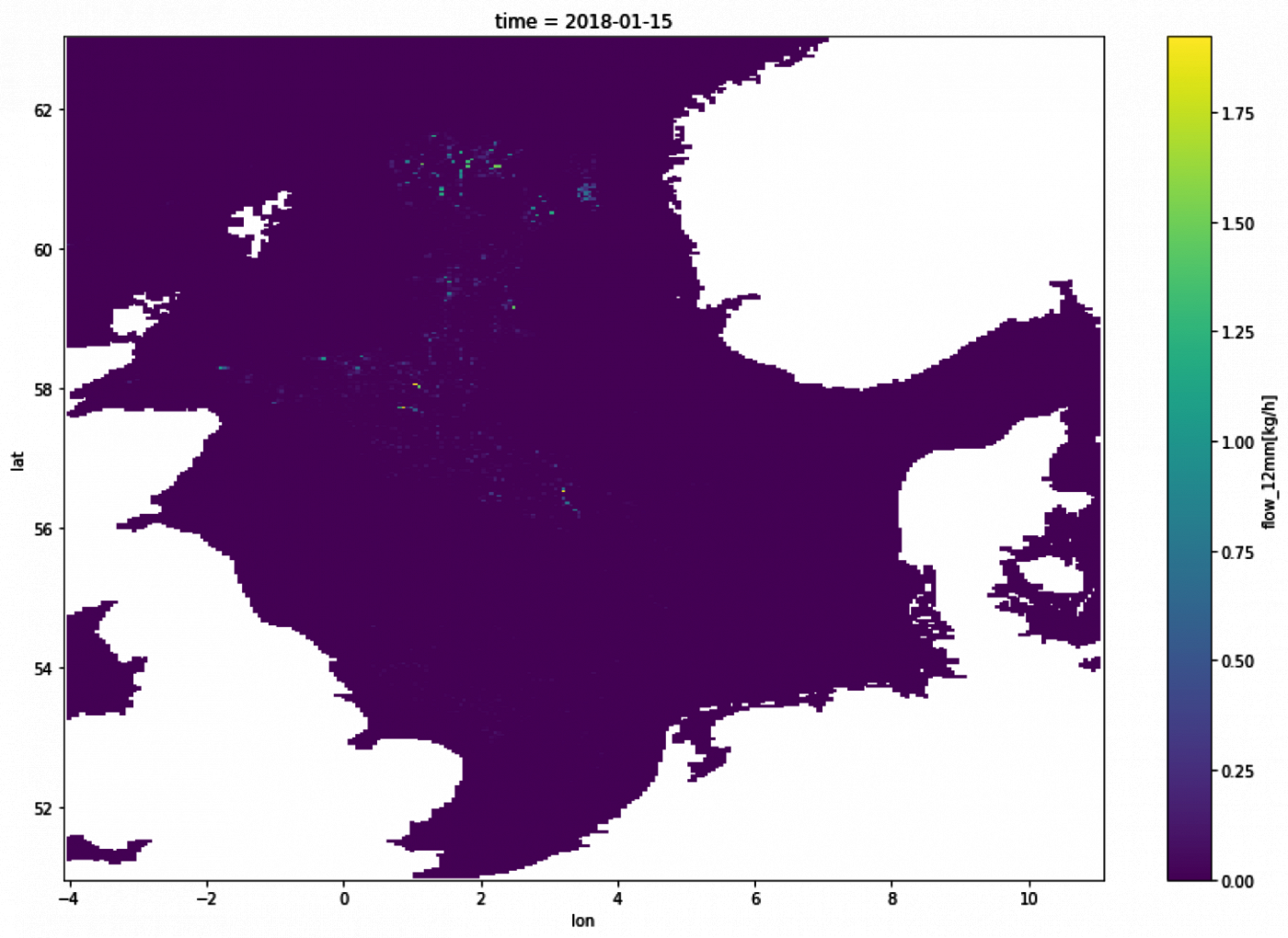
The “Concentration Map” covers the entire study area and aggregates the flow rates from the individual wells. On the image to the right you can see an exemplary output for the flow of 12mm bubbles (1l/h) to the water column below the pycnocline during the second week of 2018.
Lateral Transport
The water in the North Sea is not stationary but constantly moving. This leads to a spreading of the dissolved methane in the water column. To model this movement, we use the currents given in the NEMO model and the Lagrangian framework OceanParcels. This allows us to investigate the spread of methane below the water column and is a crucial tool for the analysis of our model with respect to measured data.
On the right-hand side you can see an example of the zonal current (east-west direction) in the first week of 2018 above the pycnocline.
References:
- The Parcels v2.0 Lagrangian framework: new field interpolation schemes - Delandmeter, P and E van Sebille (2019), Geoscientific Model Development, 12, 3571–3584
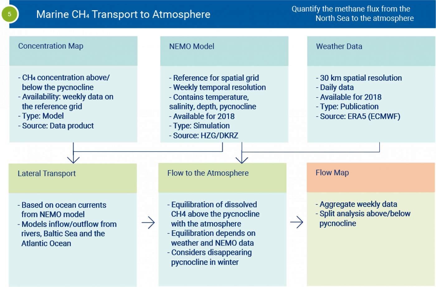
Flow to the Atmosphere
In general, in our model the flow to the atmosphere is equivalent to the flow above the pycnocline from the „Flow Map“. However, the changing composition of the water column needs to be accounted for. We therefore adapt the model to account for changes in the water column. The most prominent change is the disappearance of the pycnocline. This can happen during storms due to the shallowness of the North Sea. We therefore account to the changes in the pycnocline level by adjusting the methane flow to the changing conditions. For the locations of the wells alone, this is not a major change. We however combine this with the lateral transport model and add the effect for additional grid cells without well locations.
Flow Map
The “Flow Map” is an updated version of the “Concentration Map” with the adjustment from the “Lateral Transport” step and the “Flow to the Atmosphere” step. It therefore combines direct flow from the previous workflow with the adjustments from this workflow. The shape stays the same as for the “Concentration Map”. It is a weekly dataset covering the North Sea using the NEMO reference grid.
5) CH4 Predictions Using ML
Machine learning methods predicting temporal and spatial variations of CH4 using weather conditions and proxy variables (CO,C2H4)
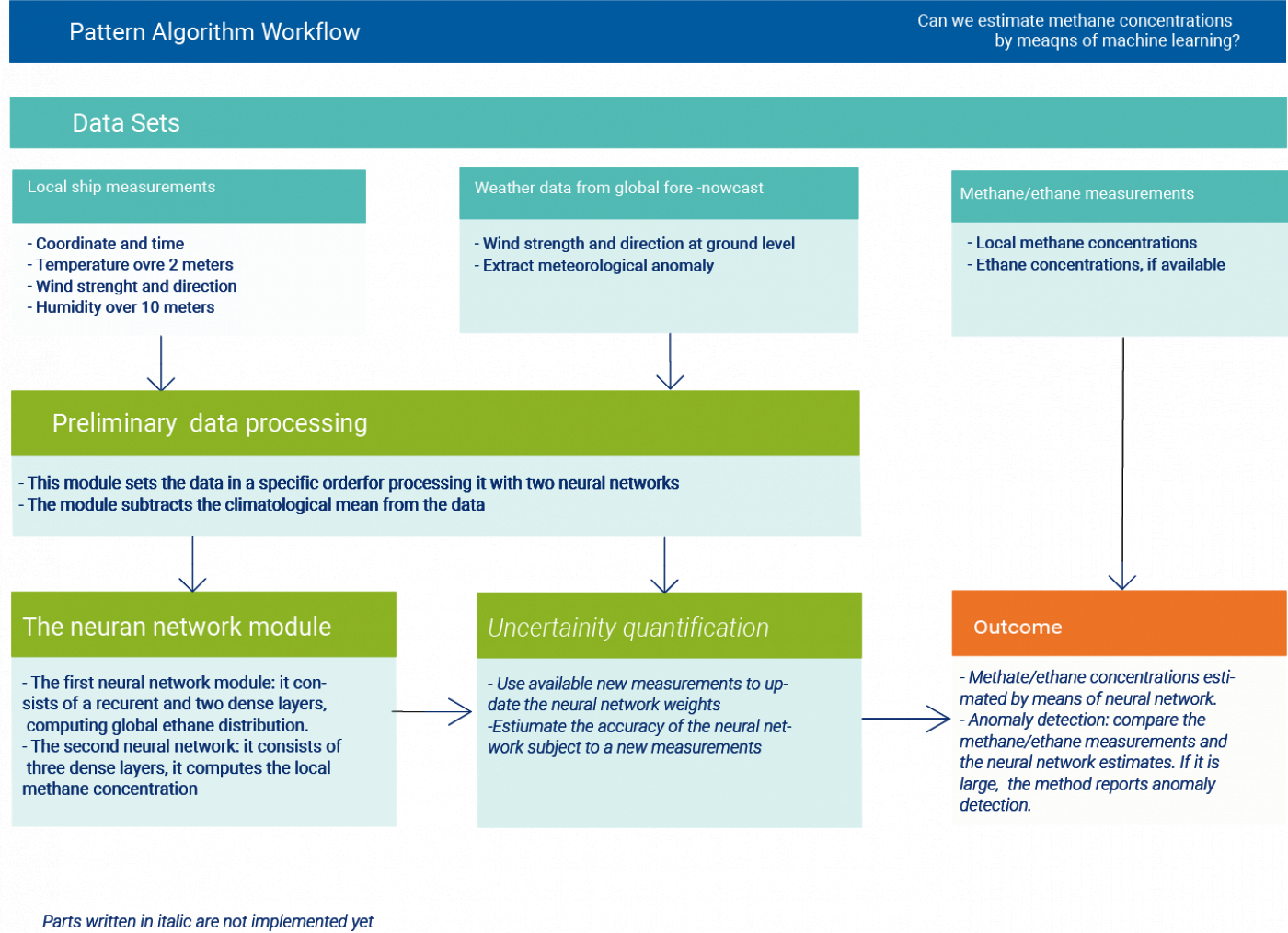
1) Estimation of methane concentration using machine learning
We aim to estimate methane concentrations near the oil and gas fields using neural networks. According to (Weber et al. 2019.), the neural network builds nonlinear empirical models estimating methane concentrations, based on its relationship to the predictor variables, plausibly linked to CH4 distribution in the atmosphere.
The selection of predictors is at the developer's choice. These can be any variables on which methane concentration depends. The neural network is adjusted on a known set of predictors and methane concentrations by fitting its computations to the corresponding observations. We select geographical coordinates, temperature, wind, and time as predictors.
Note that oil and gas fields are the unique sources of methane with certain geographic coordinates. A neural network links methane concentration produced by these sources to a geographical location by analyzing the previously observed data. Therefore, it is a priori aware of the location and strength of the sources. Similarly, analyzing methane concentrations at different points in time can detect the effects of tides and transport processes from meteorological data.
2) Estimation of ethane concentration as a proxy for methane using machine learning
The first neural network can estimate only the local anomalies in methane concentration measurements near the oil fields in the North Sea basin. However, it cannot determine whether the gas came from the oil field or has other sources. To exclude the impact from other sources, we developed the second neural network, approximating the ethane estimates of the Consortium Multiscale Air Quality Model (CMAQ) (Byun and Schere 2006) in the European domain. This neural network computes the fraction of ethane originating aside from the oil field using wind velocity as inputs. Note that leaking natural gas contains up to several presents of ethane, and it is the major source of atmospheric ethane. The concentration ratio ethane/methane is unique for each oil or gas field and preserves in time, serving a kind of fingerprint. Using this ratio and ethane estimates from the second neural network, we can compute the fraction of methane not related to the oil fields.
References:
- Byun, D., Schere, K.L., 2006. Review of the Governing Equations, Computational Algorithms, and Other Components of the Models-3 Community Multiscale Air Quality (CMAQ) Modeling System. Appl. Mech. Rev. 59, 51–77.
Methane Estimates using ML
We aim to estimate methane concentrations near the oil and gas fields using neural networks. According to (Weber et al. 2019.), the neural network builds nonlinear empirical models estimating methane concentrations, based on its relationship to the predictor variables, plausibly linked to CH4 distribution in the atmosphere.
The selection of predictors is at the developer's choice. These can be any variables on which methane concentration depends. The neural network is adjusted on a known set of predictors and methane concentrations by fitting its computations to the corresponding observations. We select geographical coordinates, temperature, wind, and time as predictors.
Note that oil and gas fields are the unique sources of methane with certain geographic coordinates. A neural network links methane concentration produced by these sources to a geographical location by analyzing the previously observed data. Therefore, it is a priori aware of the location and strength of the sources. Similarly, analyzing methane concentrations at different points in time can detect the effects of tides and transport processes from meteorological data.
References:
- Weber, T., Wiseman, N.A. & Kock, A. Global ocean methane emissions dominated by shallow coastal waters. Nat Commun 10, 4584 (2019). https://doi.org/10.1038/s41467-019-12541-7
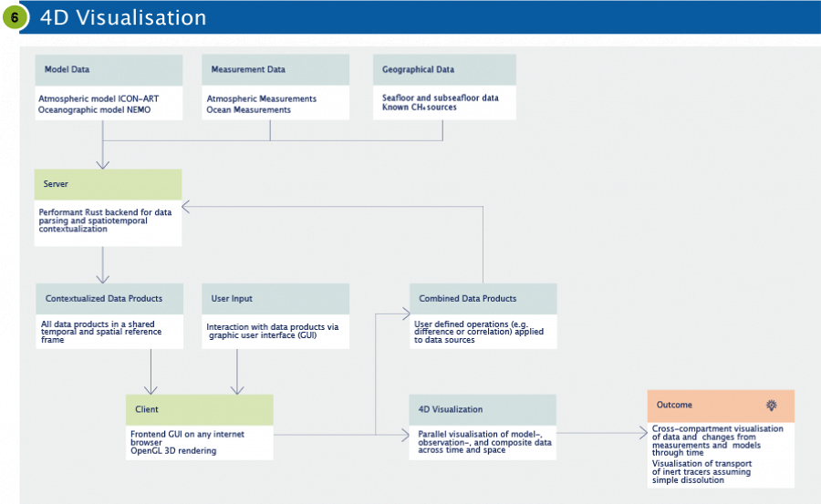
6) 4D Data Visualization
The Digital Earth showcase “Methane Budget in the North Sea” makes use of the Digital Earth Viewer to unify a large number of datasets under a single visualisation interface.
The GEBCO1 bathymetric data for the North Sea region is displayed in a 3D elevation model. The aerosol and trace gases dispersion model ICON-ART (Rieger et al. 2015) is used to calculate the contribution of different methane sources to the atmospheric methane concentration. The viewer’s interface allows to quickly compare the resulting data product with existing methane estimates from the EDGAR database2 and provides a visual corroboration of their accuracy. In a similar way, measurements of geochemical water properties are displayed in spatial context of other measurement compilations from the Pangea3 and MEMENTO (Bange and Bell 2009) databases. The observation of their development over time is further supported by the visualization of three-dimensional physical water properties like current velocities and pycnocline depth obtained from the NEMO Model (Madec et al. 2019).
This parallel visualization of multiple data and information sources is unique in the field of Earth and Environment and greatly supports the users in building mental models and the subsequent communication of them to scientific users.
References:
- D. Rieger et al. 2015, ICON–ART 1.0 – a new online-coupled model system from the global to regional scale. Geosci. Model Dev., 8, 1659–1676.
- Bange, H. W., and T. G. Bell (2009), MEMENTO: A marine methane and nitrous oxide database, Solas News, Issue 9, Spring 2009, page 42.
- Gurvan Madec and NEMO System Team (2019), NEMO ocean engine. Scientific Notes of Climate Modelling Center (27) – ISSN 1288-1619
Links:
7) Data Exploration for Marine CH4
To evaluate the performance of our model and to find adequate parameters for flow and bubble size distribution, we compare the model data to measurement data. The measurement data we collected covers both the water column and the atmosphere.
We use data analysis techniques to identify traces of methane in the measurement data using the model as a reference for areas where we expect to see excess methane compared to other areas. The model data is corrected for external sources of methane which might influence the concentrations in our study area. For the comparison we rely on computational and visual approaches. Computed difference maps are analyzed in the difference explorer.
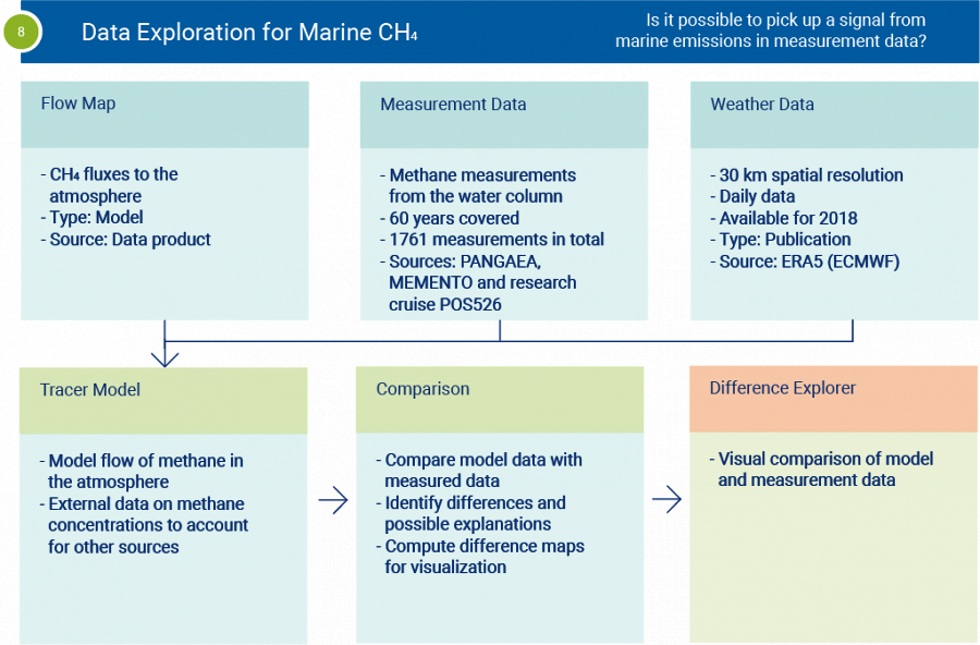
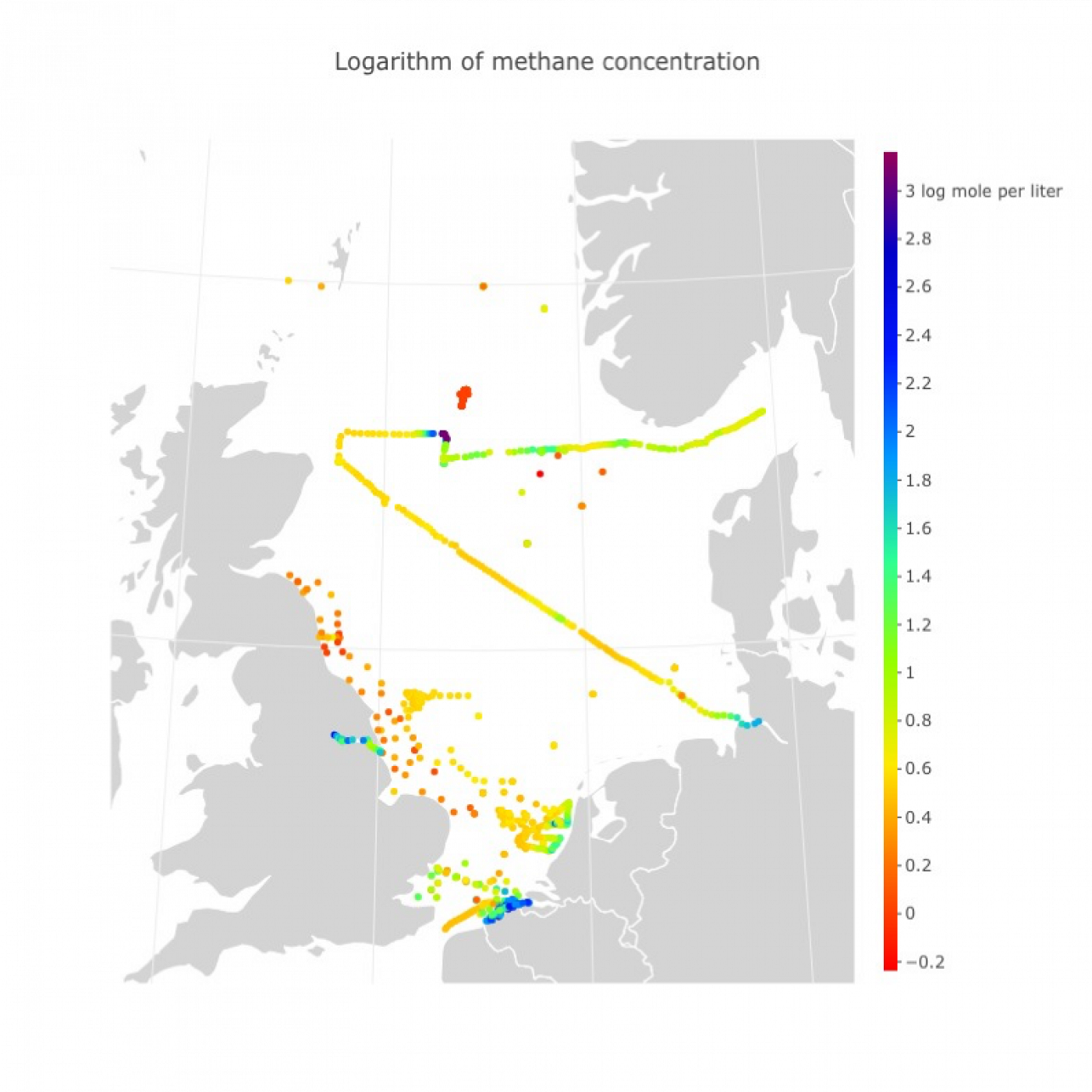
8) Measurement Data
We collected a dataset with methane measurements in the water column by combining various dataset from PANGAEA and the MEMENTO database. These measurements were collected during the past sixty years (while a majority has been collected more recently). With these measurements the modeled flows to the water column can be analyzed. On the right-hand side you can see a map of the collected measurements. Overall we have 1761 measurements.
In addition to that we have atmospheric measurements from a few research cruises in the North Sea. With these measurement we can analyze the methane flow going to the atmosphere (or water column above the pycnocline which is equivalent in our approach).
References:
- Bange, H. W., et al. (2009), MEMENTO: A proposal to develop a database of marine nitrous oxide and methane measurements, Environmental Chemistry, 6, 195-197. (https://memento.geomar.de/de)
- PANGAEA Data Publisher for Earth & Environmental Science (https://www.pangaea.de/)
Tracer Model
The “Tracer Model” can be seen as the atmospheric equivalent to the “Lateral Transport” model which is for the ocean. To connect the measurement data with the modeled methane flow, we can not only rely on measurement at well locations due to the low number of measurements. We therefore use the information from the weather data to model the wind using OceanParcels. This way we try to identify traces of methane in measurement data.
References
- The Parcels v2.0 Lagrangian framework: new field interpolation schemes - Delandmeter, P and E van Sebille (2019), Geoscientific Model Development, 12, 3571–3584
Comparison
The comparison of measurement data and our model data consists of two elements. The first element is the analysis of the influence of the flow in the model. This approach should essentially determine the necessary flow to create clear signal for our measurement locations. To do so we vary the flow rate and investigate the changes of the “Flow Map” and “Tracer Model” at measurement locations.
The second element is data analysis based. By using an aggregated ocean model we investigate the whether there are trends of increased methane concentration “down current” from well locations.
Difference Explorer
The idea of the “Difference Explorer” is to visualize the surplus methane in the water column and the atmosphere and compare it to measurement data. Here the focus is not on the absolute levels, but on the additional methane, for example down wind from a well or “down current” in the water column. Using different
For the implementation we again rely on the available frameworks in the Digital Earth project.
References:
- Grunwald et al., 2009: doi:10.1016/j.ecss.2008.11.021
- Rehder et al., 1998: doi.org/10.1023/A:1009644600833
- Römer et al., 2017: doi:10.1002/2017GC006995
- Mau et al., 2015: doi.org/10.5194/bg-12-5261-2015
- Schneider v. Deimling et al., 2011, doi:10.1016/j.csr.2011.02.012
- McGinnis et al., 2006: doi:10.1029/2005JC003183
- Matoušů et al., 2019, doi.org/10.1007/s00027-018-0609-9